Table of Contents
This is going to be a short article/tutorial on how to implement GPU-accelerated cellular automata. Quick disclaimer: please note that, while employing GPU for this task is fun, it certainly isn't the fastest approach. If you want to get real fast simulation, go ahead and checkout hashlife/golly links in the "Further reading" section.
We will start with brief introduction to cellular automata, GPU shaders, and why they are useful for CA simulation, and then move on to step-by-step description of relevant parts of ARB_fragment_program OpenGL extension and further. Basic OpenGL knowledge is required for better reading experience.
Cellular automaton (CA) is by definition a periodic grid of cells, where in each cell sits a finite automaton, and a set of (identical) rules for every such automaton describing to which state it switches on a next moment of discrete time ti+1, depending of its own state and states of all its neighbors on a current moment of time ti. For now, we will be interested in 2d, rectangular CA, and a neighborhood which includes 8 neighbors of the cell. This is what is called the Moore neighborhood, because it was invented by Edward Moore.

Of course, such rectangular 2d cellular automata are easy to visualize: we just draw each cell as a single pixel, colouring it according to the cell's state.
This description is probably enough for the sake of this article, but if you fell like you need more, you might want to check out wikipedia article.
Note
Another, funkier neighborhood type exists, called Margolus neighborhood, which is out of our scope for now, but stay tuned, since I plan to address it in another post.
Now to the shaders part. Shader is essentialy a GPU program describing what manipulations we want to perform on every pixel (or a vertex, but we're interested in pixels for now), before said pixel is sent further down the GPU pipeline. Important characteristic of this program is that all the pixels mutate independently of each other (we can imagine the process as if every pixel is handled in parallel with all others).
There is an OpenGL extension, called ARB_fragment_program, which defines a set of low-level instructions for shader programming. Nowadays, this extension is supported by virtually every GPU on the market, and this is what we are going to use in this tutorial. Here is how a very simple program on the assembly language defined by this extension (I will refer to it as to ARB assembler language, or ARB for short) looks like:
Example 1. Simple ARB program, drawing pixels as-is
!!ARBfp1.0                                     # standard ARB header
TEMP cur_clr;                                  # variable "cur_clr" declaration
TEX  cur_clr, fragment.texcoord, texture, 2D;  # put texture sample corresponding to the current fragment to cur_clr
MOV  result.color, cur_clr;                    # define resulting color for the current fragment
END                                            # everything except "cur_clr" here are standard keywords
We will continue composing ARB programs learning needed instructions and concepts on the fly, but if you feel like you need a somewhat deeper explanation first, I suggest a wikipedia article on the subject, ARB (GPU assembly laguage), it's pretty good. Also, here is a very thorough (but not too user-friendly) ARB_fragment_program specification. I find sections 3.11.4 and 3.11.5 there to be particularly useful.
To think about it, these shader programs are exactly what we need for CA simulation - remember, in CAs, each cell state at the moment ti+1 depends upon whatever states at the moment ti, but never depend on the state of any cell at the very same moment ti+1. And this kind of data parallelism is exactly how shaders work.
We will now proceed to learn how to write shader programs in ARB assembly language, load the program into the GPU, compile it and render a simple scene, effectively simulating 2 simple CAs, all using OpenGL API.
Here is an outline of general structure of the program:
-
Create a texture holding an initial state of CA lattice (cell state is encoded as pixel color)
-
Load shader program to the GPU and compile it
-
Draw the scenery using the texture and applying the shader program (this does a single step of the simulation)
-
Retreive resulting image from frame buffer and store it in the texture (using
glCopyTexImage2D()) -
Repeat from step 3
Since we want every single pixel on a texture to be processed by the shader program, we need to construct the scenery properly. Easiest way seems to be to create 1:1 mapping between on-screen pixels and texture texels:
Example 2. Viewport and projection matrix initialization
gl.glViewport(0, 0, TEX_WIDTH, TEX_HEIGHT);  // set the viewport's size to the texture size

gl.glMatrixMode(GL.GL_PROJECTION);
GLU glu = new GLU();
glu.gluOrtho2D(-1, 1, -1, 1);                // set 2d orthographic projection as a projection matrix

gl.glMatrixMode(GL.GL_MODELVIEW);            // set the identity matrix as a modelview matrix
gl.glLoadIdentity();
Note
I'm using Java OpenGL bindings (jogl) here, but all this is nearly identical in other languages. Here is a good resource to look up OpenGL (and others) API: http://start.gotapi.com/.
In the projection we just created, if you draw a single quad with coordinates (∓1, ∓1,
-0.5), it occupies the whole viewport. And if you stretch a texture of size (TEX_WIDTH, TEX_HEIGHT) onto it, every texel will occupy a single pixel on the screen:
Example 3. Scenery-drawing code
gl.glBegin(GL.GL_QUADS);
{
  gl.glTexCoord2f(0, 0);                     // assign (0, 0) texture corner to
  gl.glVertex3f(-1, -1, -0.5f);              // (-1, -1) quad corner
  gl.glTexCoord2f(1, 0);                     // etc.
  gl.glVertex3f(1, -1, -0.5f);
  gl.glTexCoord2f(1, 1);
  gl.glVertex3f(1, 1, -0.5f);                // Z coordinate is chosen arbitrarily
  gl.glTexCoord2f(0, 1);
  gl.glVertex3f(-1, 1, -0.5f);
}
gl.glEnd();                                  // the quad is drawn with the texture stretched over it
gl.glFlush();
Also, since we need to retreive resulting image on each step and use it as the texture on the next step, we
might need to disable some of the fancy features such as lighting, blenging, magnification/minification texture
filters and others. I'm not sure about the completeness of the list of features to disable, but this seems to
work fine for me:
Example 4. OpenGL features and texture initialization
disable(gl, GL.GL_LIGHTING);                          // disable various unnecessary features
disable(gl, GL.GL_LIGHT0);
disable(gl, GL.GL_BLEND);
disable(gl, GL.GL_DEPTH_TEST);

enable(gl, GL.GL_TEXTURE_2D);                         // enable textures usage

int[] _textures = new int[1];
gl.glGenTextures(1, _textures, 0);                    // request one texture to be created, id is stored in _textures[0]
reportError(gl);                                      // check for possible errors and handle them

gl.glBindTexture(GL.GL_TEXTURE_2D, _textures[0]);     // set the texture in operation
reportError(gl);                                      // don't you ever forget this

gl.glTexParameteri(GL.GL_TEXTURE_2D, GL.GL_TEXTURE_MIN_FILTER, GL.GL_NEAREST); // here goes actual fancy features disabling
gl.glTexParameteri(GL.GL_TEXTURE_2D, GL.GL_TEXTURE_MAG_FILTER, GL.GL_NEAREST);
gl.glTexParameteri(GL.GL_TEXTURE_2D, GL.GL_TEXTURE_WRAP_S, GL.GL_CLAMP);
gl.glTexParameteri(GL.GL_TEXTURE_2D, GL.GL_TEXTURE_WRAP_T, GL.GL_CLAMP);

FloatBuffer buf = createInitialTexture();             // create a buffer with initial CA state
gl.glTexImage2D(GL.GL_TEXTURE_2D, 0, GL.GL_RGBA8,
                TEX_WIDTH, TEX_HEIGHT, 0, GL.GL_RGBA,
                GL.GL_FLOAT, buf);                    // initialize the texture with the buffer
reportError(gl);
Initialization of the ARB program in general looks like this:
-
Enable FRAGMENT_PROGRAM_ARB extension
-
Request program object to be created, get an id and bind it
-
Load the actual program in the textual form and compile it
-
Set up any external parameters to pass to the program
-
Use it while rendering
Here is how it is being done with jogl:
Example 5. ARB program initialization
enable(gl, GL.GL_FRAGMENT_PROGRAM_ARB);               // enable the extension

int[] _programs;
gl.glGenProgramsARB(1, _programs, 0);                 // request internal program object to be created, _programs[0] holds the id
reportError(gl);                                      // handle errors if any

gl.glBindProgramARB(GL.GL_FRAGMENT_PROGRAM_ARB,
                    _programs[0]);                    // select program object to be used from now on
reportError(gl);

StringBuilder b = readProgramFromFile(fileName);
gl.glProgramStringARB(GL.GL_FRAGMENT_PROGRAM_ARB,     // try to compile the program
                      GL.GL_PROGRAM_FORMAT_ASCII_ARB,
                      b.length(), b.toString());
if (gl.glGetError() != 0) {
  // if the compilation failed, see at which line it happened:
  int pos[] = new int[1];
  gl.glGetIntegerv(GL.GL_PROGRAM_ERROR_POSITION_ARB, pos, 0);
  // report and handle...
}
I will also pass an external parameter to the ARB program (it will prove useful later):
Example 6. ARB program parameter passing
// every parameter is a 4d float vector
gl.glProgramEnvParameter4fvARB(GL.GL_FRAGMENT_PROGRAM_ARB, 1,
                               new float[] {  1.0f / (float)ARBdemo.TEX_WIDTH, 0.0f,
                                             -1.0f / (float)ARBdemo.TEX_WIDTH, 0.0f },
                               0);
What I pass above as a parameter is the distance between two adjacent pixels on the texture, so that ARB
program would know what is the current texture size. Also, since we're going to use rectangular texture, I
didn't use TEX_HEIGHT here.
So far, we've been talking mainly about the structure of a "wrapper" program (int this case, written in Java), not the ARB program itself, which should do all the CA simulation work. Now it's time to look at the parts of the ARB program which are generic for all CAs using Moore neighborhood.
We already
know how to address the current texel, but in order to work with Moore neighborhood, we'd also need to know
how to address all the neighbors. Texture coordinates are float values in the range of [0.0,
1.0] (remember, how we
mapped a texture to a quad?). That is, if we have e.g. a texture of 512 width, we
will refer to texel's X coordinate in the ARB program as to [0,
1/512, 2/512, ..., 1-2/512, 1-1/512]. So, it turns out, we need to know the texture's dimensions in the
ARB program. This is where passed parameter comes handy:
Example 7. Addressing neighbor (+1, 0) in ARB program
TEMP shift;                                  # 4d float vector holding shift distances for adjacent texels
MOV  shift, program.env[1];                  # e.g. when TEX_WIDTH=512, shift = (1/512, 0, -1/512, 0)
                                             # shift.x serves as positive shift, shift.z - negative one

TEMP cur_pos;                                # variable to hold neighbor coordinates
ADD  cur_pos, fragment.texcoord, shift.xwww; # ADD does parallel addition of all 4 components
                                             # shift.xwww = (shift.x, shift.w, shift.w, shift.w) = (1/512, 0, 0, 0)
                                             # so cur_pos = (fragment.x+1/512, fragment.y, fragment.z, fragment.w)

TEMP cur_clr;                                # now we can retrieve color of the neighbor texel:
TEX  cur_clr, cur_pos, texture, 2D;
One more thing, let's make our simulation world toroidal, because it is good to know that the world is self-contained. Torus is preferable to sphere, because:
-
There are no deformation when unfolding torus to a 2d surface (i.e. the screen)
-
Required "wrapping" is embarrassingly easy to implement
Since torus unfolds to a rectangle, all we need to do is to solder left/right edges of the texture together and do the same with top/bottom edges. E. g. when we are retrieving a value of a neighbor beyond the left edge, we should get rightmost texel on the same row instead:
Example 8. Wrapping over the left edge, neighbor (-1,
0)
TEMP max_coord;                                  # define maximum coordinate any texel could have
SUB  max_coord, 1, shift.x;                      # max_coord = (M, M, M, M), where M = 1 - 1/512

ADD  cur_pos, fragment.texcoord, shift.zwww;     # cur_pos = (x-1/512, y, z, w)
CMP  cur_pos.x, cur_pos.x, max_coord, cur_pos.x; # check if we need to wrap X coord around - the CMP is equivalent to:
                                                 # cur_pos.x = cur_pos.x<0 ? max_coord : cur_pos.x;
TEX  cur_clr, cur_pos, texture, 2D;
Similarly done is wrapping over the bottom (for example) edge:
Example 9. Wrapping over both left and bottom edges, neighbor (-1,
+1)
TEMP ge_512;                                     # this will serve as a boolean flag where 1.0 represents true

ADD  cur_pos, fragment.texcoord, shift.zxww;     # cur_pos = (x-delta, y+delta, z, w)
CMP  cur_pos.x, cur_pos.x, max_coord, cur_pos.x; # left wrapping, adjusting X coord
SGE  ge_512, cur_pos.y, 1;                       # check if we need to wrap Y, SGE is equivalent to: ge_512 = cur.pos.y >= 1;
CMP  cur_pos.y, -ge_512, 0, cur_pos.y;           # cur_pos.y = -ge_512<0 ? 0, cur_pos.y
TEX  cur_clr, cur_pos, texture, 2D;
I suspect it is common knowledge already, but anyway... This cellular automaton, also called The Game of Life, has the following simple rules:
-
Each cell has only 2 states, active and passive
-
If an active cell has less than 2 or more than 3 active neighbors, it becomes passive on the next step
-
If a passive cell has exactly 3 active neighbors, it becomes active on the next step
I encourage you to explore the references section to find out how amazingly reach is the world of configurations spawned from this simple rule set.
In ARB assembly, every pixel color is a 4d float vector which components can be refeered to as (r, g, b, a). Suppose we represent an active cell as a pixel of (1, 1, 1,
1) color, and a passive one as (0, 0, 0, 0) color. Obviously, to implement the
Life rule set, we'll need to calculate the number of active neighbors. Here is how we do it:
Example 10. Calculating number of active neighboring cells
TEMP is_active;                                  # is_active acts as a boolean (but still is a 4d float vector)
TEMP num_neigh;                                  # variable holding the number of active neighbors
MOV  num_neigh, 0;                               # init with zero, num_neigh = 0

ADD cur_pos, fragment.texcoord, shift.xwww;      # get (+1, 0) neighbor coordinates
  SGE ge_512, cur_pos.x, 1;                      # wrap X coordinate over the torus edge if needed
  CMP cur_pos.x, -ge_512, 0, cur_pos.x;
TEX cur_clr, cur_pos, texture, 2D;               # get neighbor color
                                                 # let's check only R component of color
SGE is_active, cur_clr.rrrr, 0.6;                # is_active = (r>0.6, r>0.6, r>0.6, r>0.6)
ADD num_neigh, num_neigh, is_active;             # num_neigh is increased by 1, if is_active is set

# continue like this for the rest 7 neighbors
# in the end, num_neigh holds the number of active neighbors
Now, knowing how many active cells are around, the subsequent state of the center cell depends on its own state
at the current moment. ARB assembly language doesn't have a notion of conditional branching, so we will have to
settle with conditional move instead:
Example 11. Setting the cell's state based on current state and number of active neighbors
TEMP num_ge;                                   # flag, used when something is < something else
TEMP num_le;                                   # same for >
TEMP new_cell;

TEMP cur_clr;
TEX  cur_clr, fragment.texcoord, texture, 2D;  # get current cell state

# first, let's check if a passive cell should become an active one
TEMP new_cell;                                 # check for equality is done with two comparisons: <= and >=
SGE  num_ge, num_neigh, 3;                     # num_ge = num_neigh>=3 ? 1 : 0;
SGE  num_le, -num_neigh, -3;                   # num_le = num_neigh<=3 ? 1 : 0;
SUB  new_cell, 1, cur_clr.rrrr;                # new_cell = (the cell is passive) ? 1 : 0
MUL  new_cell, new_cell, num_le;
MUL  new_cell, new_cell, num_ge;               # new_cell = (N==3) && (the cell is passive)
# here new_cell is either (1, 1, 1, 1) or (0, 0, 0, 0)

# second, check if active cell should still remain active
TEMP dead_cell;
SGE  num_ge, num_neigh, 2;                     # num_ge = num_neigh>=2 ? 1 : 0;
SGE  num_le, -num_neigh, -3;                   # num_le = num_neigh<=3 ? 1 : 0;
MUL dead_cell, num_ge, num_le;                 # dead_cell = (N>=2 && N<=3)
MUL dead_cell, cur_clr.rrrr, dead_cell;        # dead_cell = (N>=2 && N<=3) && (the cell is active)
# here dead_cell is either (1, 1, 1, 1) or (0, 0, 0, 0)

# now do a conditional move depending on the current state
CMP cur_clr, -cur_clr.r, dead_cell, new_cell;  # cur_clr = (the cell is active) ? dead_cell : new_cell;

MOV result.color, cur_clr;                     # set the color of the cell for the next time step
Rule set of this CA, invented by Brian Silverman, uses Moore neighborhood and is very simple too:
-
Each cell has three possible states: passive, active, and semi-active.
-
If a cell is active, it goes to semi-active state on the next step
-
If a cell is semi-active, it becomes passive on the next step
-
If a cell is passive, it becomes active if and only if it has exactly 2 active neighbors
This resembles a simple model of neuron activation, hence the name. Unlike the Game of Life, where random patterns tend to die pretty quickly, Brian's Brain is usually very active and evolves for a huge number of iterations.
It also has interesting characteristic such as every stable structure there moves with the maximum possible
speed (so called speed of light, or c), with few exceptions:

Structure on the left moves diagonally with the speed of c/4. The right one is the only
stable and non-moving structure I'm aware of (thanks to wikipedia article; even Toffoli & Margolus were
unaware of it, it seems, at the time of the book
writing).
Since here we have 3 possible states, we will naturally encode them as (0, ...),
(0.5, ...) and (1.0, ...) colors in the shader program.
Neighbors counting then remains the same as in the Game of Life case,
because semi-active cells don't count. Knowing number of active neighbors, the only thing remaining is to
properly set up the new state:
Example 12. Brian's Brain ARB program, main part
# say, num_neigh contains the number of active neighbors

SGE num_ge_two, num_neigh, 2;                # do the usual trick when we need to check for strict equality
SGE num_le_two, -num_neigh, -2;              #
MUL new_clr, num_le_two, num_ge_two;         # new_clr = (N == 2) ? 1 : 0

TEX cur_clr, fragment.texcoord, texture, 2D; # get the current color (that would be 0.0 or 0.5 or 1.0)
SUB cur_clr, cur_clr, 0.5;                   # active -> semi-active; semi-active -> passive

# to guard from possible floating point error, so that former 0.5 won't give us <0 value after 0.5 was substracted above:
ADD tmp_clr, cur_clr, 0.25;                  # now, tmp_clr is either approx. -0.25 or 0.25 or 0.75

# if tmp_clr is <0, it means current cell was passive, and we need to put new_clr there - the result of checking for cell's activation
CMP cur_clr, tmp_clr.rrrr, new_clr, cur_clr; # cur_clr = (tmp_clr.r<0) ? new_clr : cur_clr;

# now, cur_clr, as it should be, is either 0.0 or 0.5 or 1.0
MOV result.color, cur_clr;
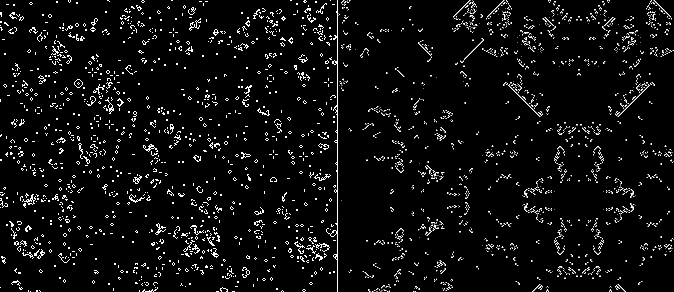
This concludes Brian's Brian ARB shader description, and here is how it usually looks like when simulating:

-
Sorry, this is not freely available book, but it's too great to be omitted from the list:
Toffoli, Margolus "Cellular Automata Machines: A New Environment for Modeling"
Excellent book on cellular automata, with physics references and examples in Fort language. One of the book's examples related to fluid dynamics refers to an article by famous Stephen Wolfram (yes, the guy who invented Mathematica and WolframAlpha.com). Here is an example of Wolfram's work on the same topic. The book also mentions a piece of hardware named "Connection Machine 1", or CM-1. Check out the next link to find out who was involved in the development of the CM-1.
-
Richard Feynman and The Connection Machine
Yep, THE Richard Feynman, worked at a start-up aimed on design of a parallel computer CM-1, back in 80s.
-
List of publications by Stephen Wolfram on the topic of cellular automata
-
An Algorithm for Compressing Space and Time
Very interesting article from Dr. Dobbs journal about amazing hashlife algorithm. Must read if you're interested in effective CA simulation.
-
Hashlife algorithm implementation and many more. Great software to play around with different CAs. And it supports infinite lattices, too.
-
Mandelbrot using ARB_vertex_program, ARB_fragment_program
Small application (with sources) for calculating the Mandelbrot set. Good as en example of what ARB_fragment_program code looks like.
-
Four-Dimensional Cellular Automata Acceleration Using GPGPU
With source code, but it's implemented on higher level C-like OpenGL Shading Language (aka GLSL), not ARB assembly language code directly.
-
A page dedicated mainly to physical application of specific CA, simulating real-life gases.
-
Hexagonal Cellular Automata Techniques
Describes several CAs similar to the Brian's Brain, on a hexagonal grid. As you might have deduced from the topic of my previous post, hexagonal grid CAs are in the list of my future write-ups too.
-
Cellular Automata Neighborhood Survey
A collection of various CA neighborhoods.
-
Eric Weisstein's Treasure Trove of The Life Cellular Automaton
Huge collection of interesting Game of Life's structures.
-
Collection of links, Life lexicon, simulator programs, etc.
Thank you for sharing it
ReplyDeletebrians club
briansclub
In today’s fast-moving digital era, platforms providing secure and reliable services are more important than ever. One such platform making waves is Brians Club, known for its innovative features and services that meet user needs. This company focuses on providing safe, efficient, and accessible digital solutions across various industries.
ReplyDelete